In this project we continue to work with warping images. Now, rather than considering affine transformations of triangles, we are considering global homographies that model changing the viewing angle while keeping the camera in the same location. We first capture multiple images from the same location, with the camera pointing in different directions. These images are all capturing the same light field, so in regions of overlap they differ only by a perspective shift, which we model as a homography The task now is to align and join the images to create an image with a wider field of view.
Homographies and Image Rectification
Before we move to image stitching, we first look at image
rectification, which is the task of applying the homography that
rectifices a selected rectangle. We compute this homography by
solving the least squares solution to a certain linear system that
describes how points transform under the homography. The key thing
here is that we are using projective coordinates which allow us to
describe how images change as the image sensor is rotated. These
projective coordinates are very interesting and connected to some
math that I would like to learn about. The equation we start with
is
[wx_i', wy_i', w] = H[x_i, y_i, 1] (*)
This is an example of computing with equivalence classes, as there
is an entire 1d subspace of R^3 that we make correspond to a single
point in R^2. From (*) we write:
x_i' = (h_11 x_i + h_12 x_j + h_12) / (h_31 x_i + h_32 x_j + h_33)
and
x_j' = (h_21 x_i + h_22 x_j + h_22) / (h_31 x_i + h_32 x_j + h_33)
Then organizing this into a system of equations, we have:
[-x_i, -x_j, -1, 0, 0, 0, x_i' x_i, x_j' x_j, x_i'] vec(H)^T = 0
[ 0, 0, 0, -x_i, -x_j, -1, x_j' x_i, x_j' x_j, x_j'] vec(H)^T = 0
Then we stack these equations to get a system that we solve by least squares.
In the case of image rectification, we can look at the case where
we have four points (x_i, x_j), and compute the homography that
takes these points to the vertices of the unit square.
Below, we look at an example of rectifying an off center rectangle:
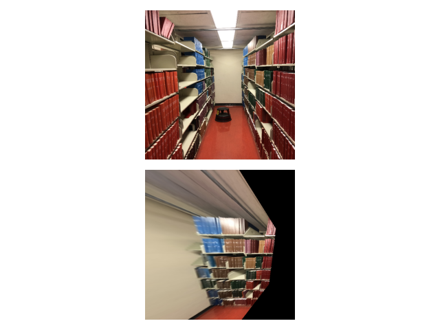
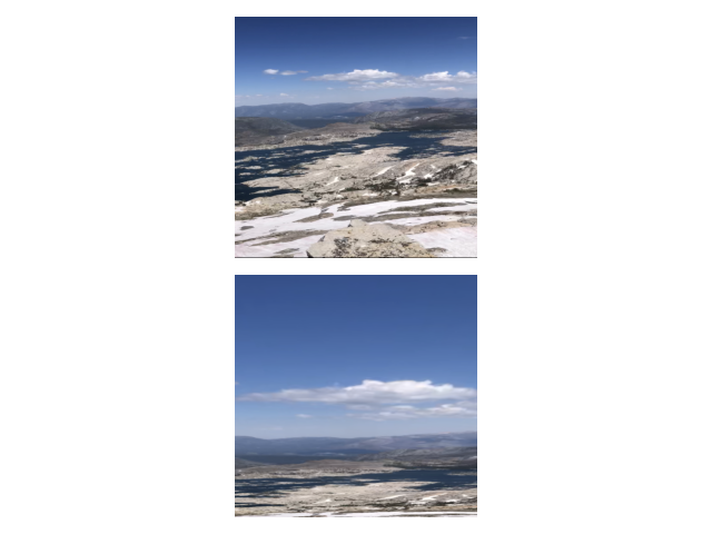
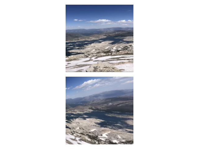
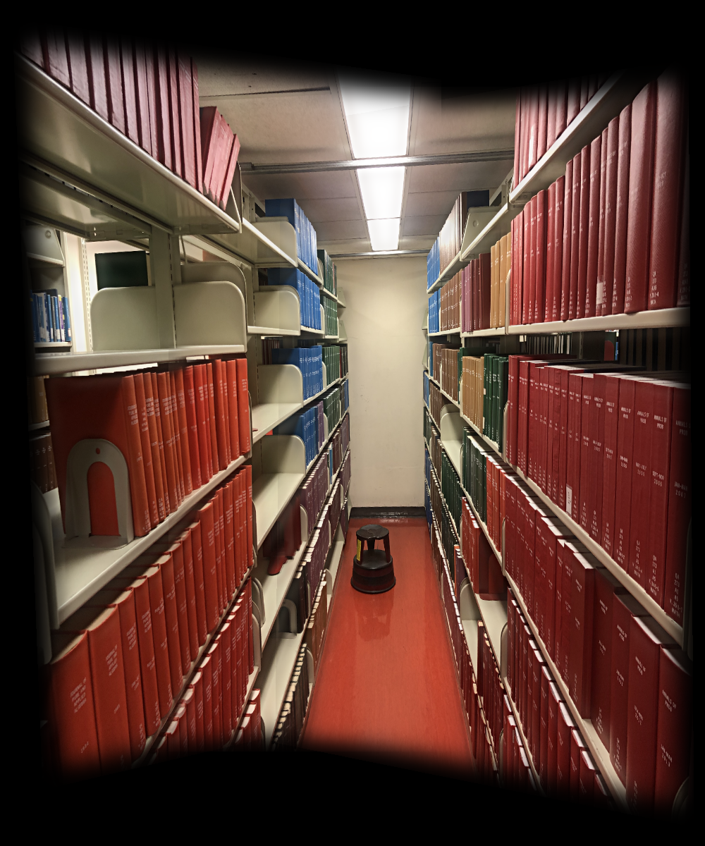
Now, we can look at taking three images and aligning them homographically so that they agree on the location of the white rectangle at then end of the aisle in the image.
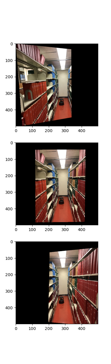
After transforming images to agree on overlapping regions, we can begin stitching the images together, using the image blending technique we developed in project 2.
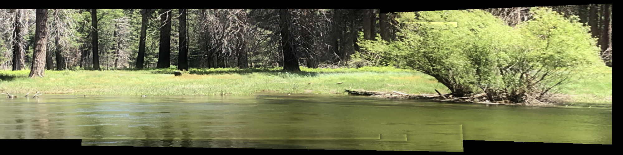
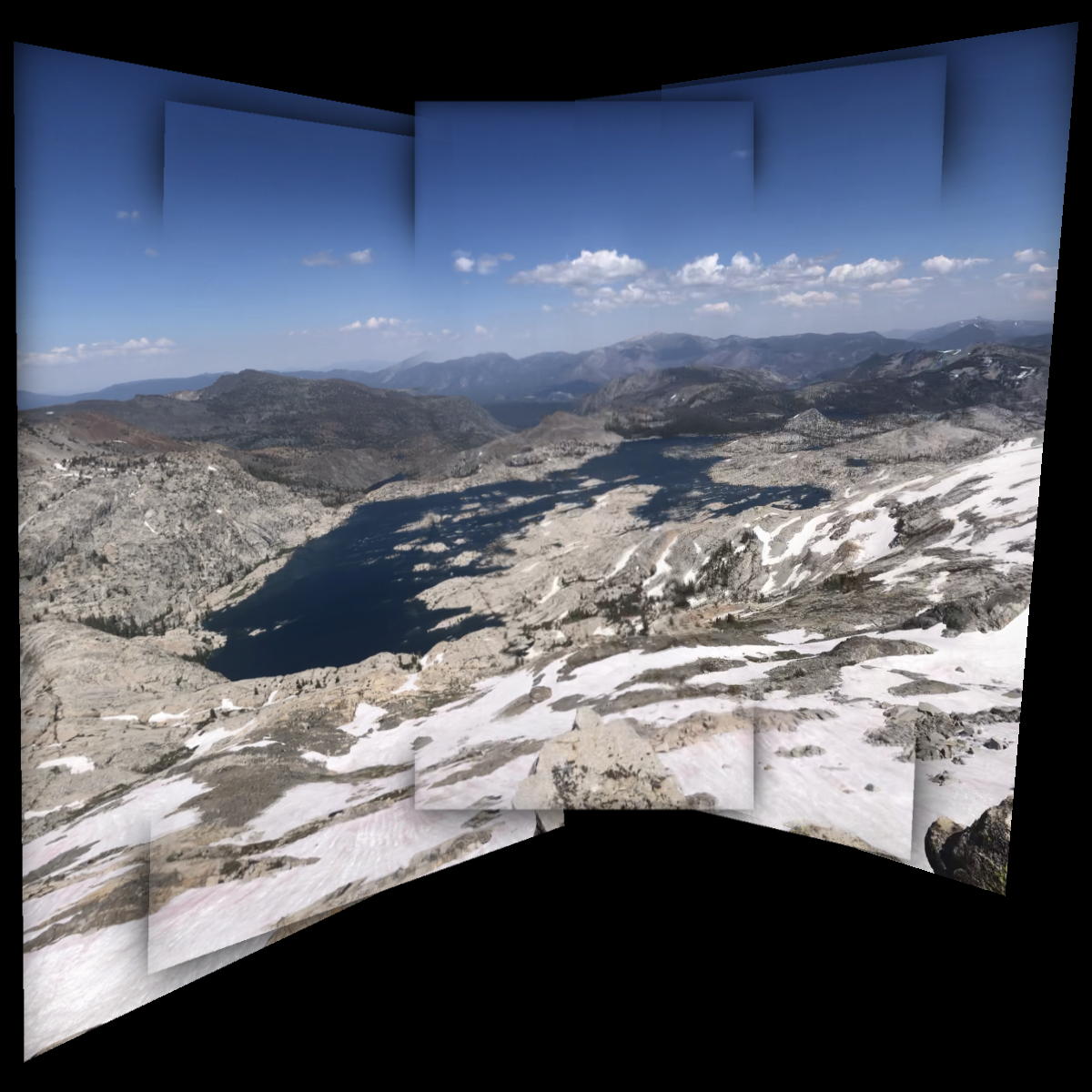
This story works for a three panel panorama, where we can clearly align the two side images to the center image. But for the case when there are an arbitrary number of images, this method becomes more challenging. Rather than aligning all images to a center image and using a notion of global coordinates, we prefer to perform the stitching iteratively, adding one new image to the stitch at a time. At each new iteration, however, we consider the current stitched image as a function from the unit square to pixel space. Thus each new iteration introduces a new coordinate system, introducing challenges for any global parameterization. When using this iterative approach, we do not need to pay attention to where the source images get mapped to in the final stitch. Rather, we warp each image to the in progress stitched image, and expand the bounds on the sampling region to accomodate for the increasing size of the stitch. The new bounds are computed by looking at where the current homography takes the corners of the unit square. When we increase the interpolation domain to include the entire image of the unit square under the homography, we ensure that the resultant stitch includes the entire new image. This can lead to problems in the case where the computed homography has high condition number, leading to the image of the unit square becoming elongated. As the bounds accomadate this, the majority of the content of the stitched image gets relegated to a small region of the final image, as shown below.
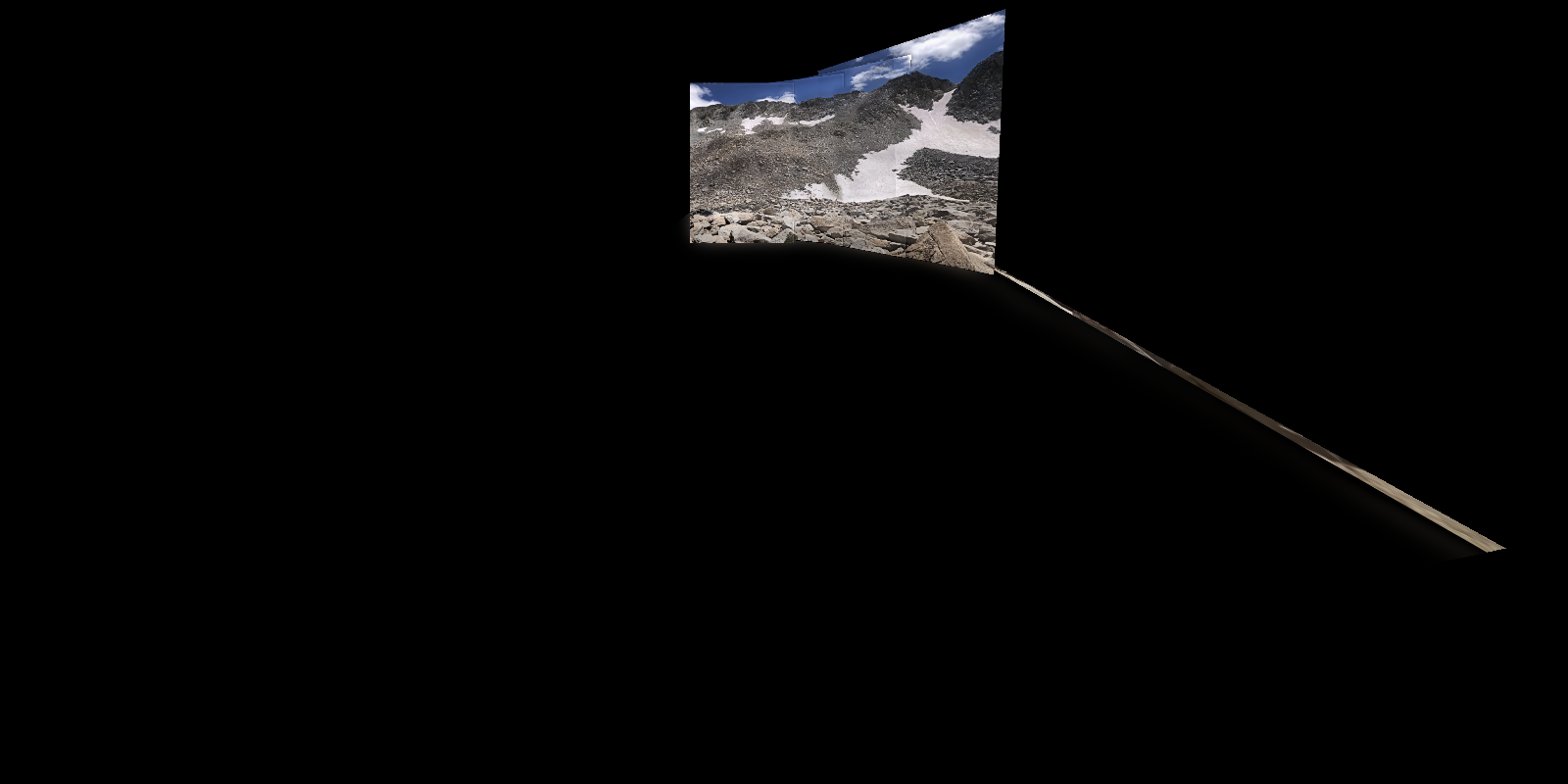
To accomadate for this, we prefer to compute homographies between images with large overlaps and small perspective changes, ensuring that the homographies are sufficiently gentle to the parts of the image that are lacking point correspondence information.
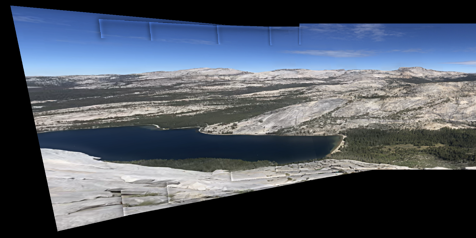
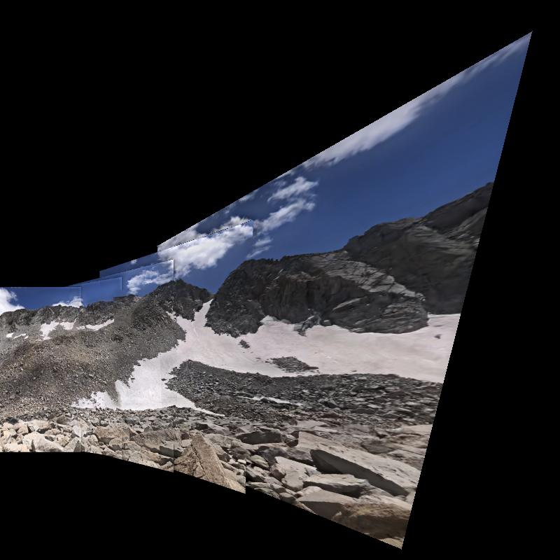
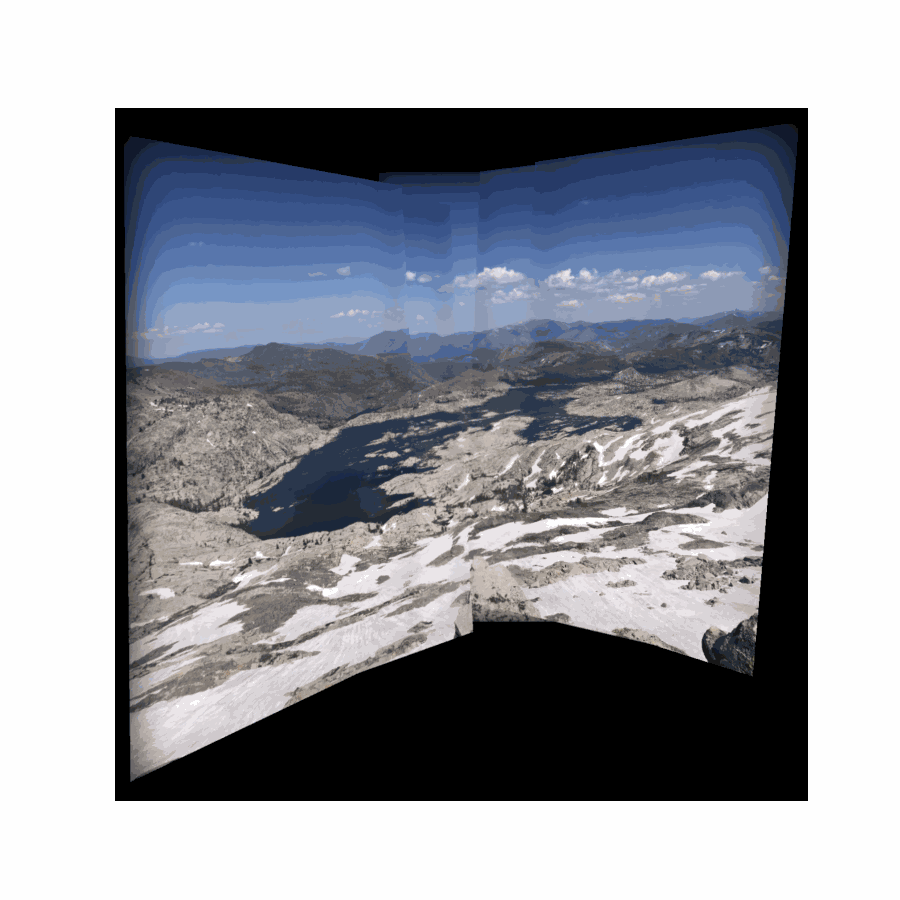
Now we see the results of a couple successfully stitched images. These stitches were made with manually selected correspondences.
I introduced various hyperparameters in the stitching code, such as epsilon tolerances to do with masks for blending, masks for updating pixels, all the hyperparameters associated with the blending (such as gaussian kernel size and standard deviation). The result is that we can achieve different blending effects depending on the different hyperparameters that we use, which result in different artifacts in the final image.
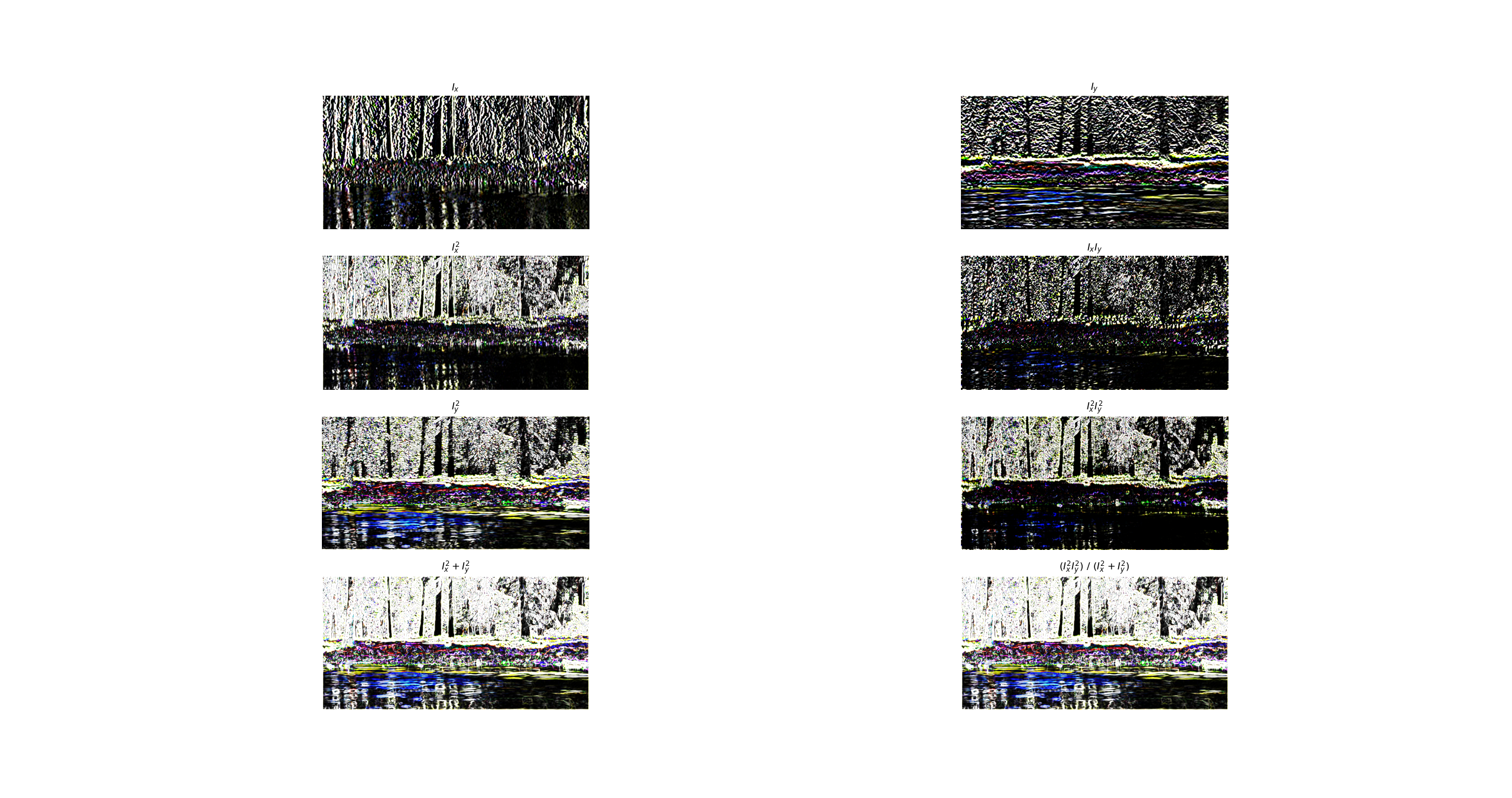
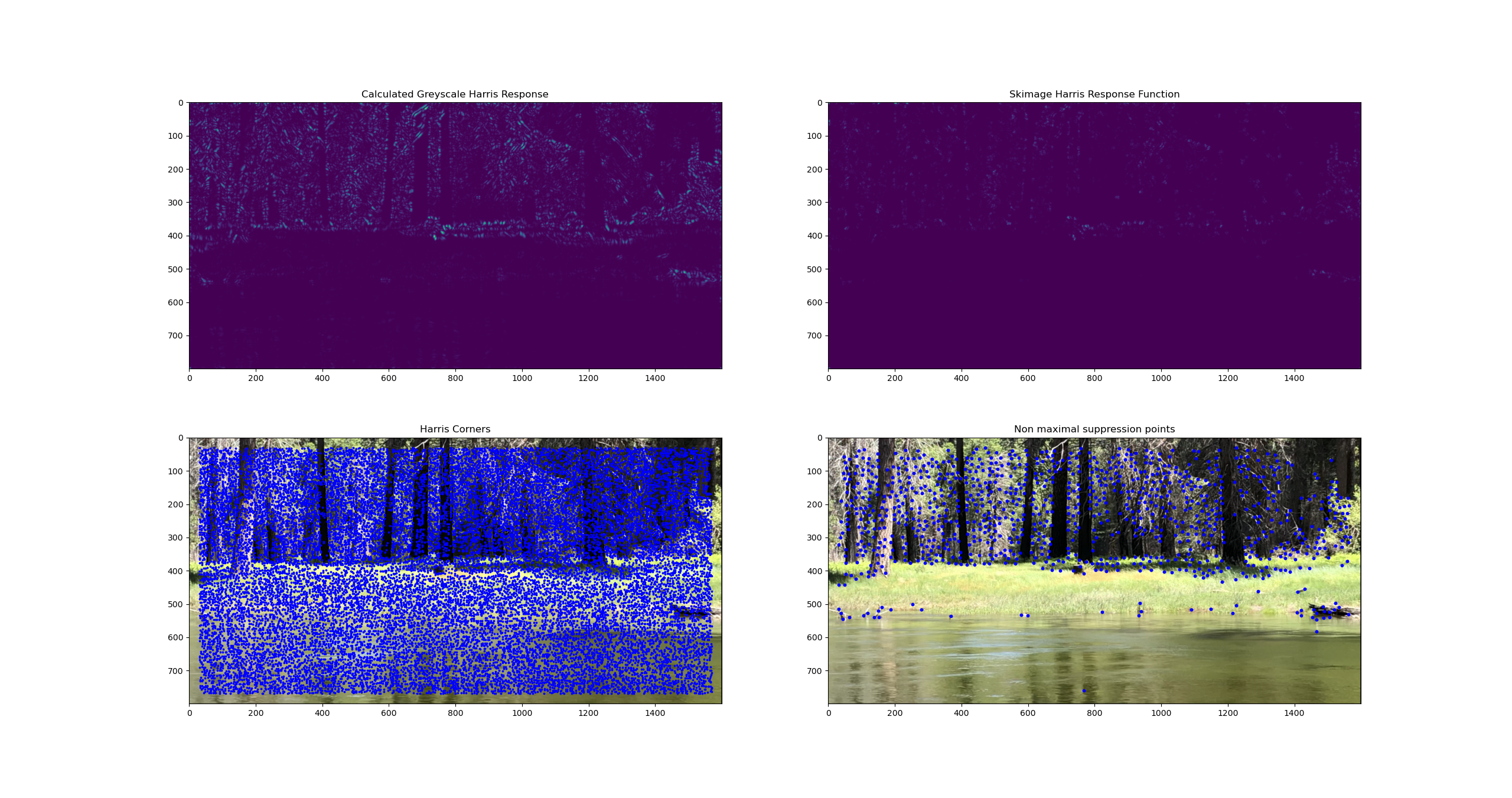
Now we tackle the task of automatically finding correspondences. Previously we manually selected the points, but this was not a robust method as it is slow and sensitive to small user errors. We first compute the harris response to our image, by taking horizontal and vertical derivatives, combining them to form the second matrix, and then computing the response as the determinant of the second moment matrix divided by its trace. In the final implementation I used the provided code that calls the skimage harris response function, but for illustration purposes I show the construction process below.
Once we have the harris response, we take the harris corners to be the points that are local maximums in their (3, 3) local neighborhoods. This gives a set of points that is too dense to work with. Next, we use Non-Maximal Suppression to select a subset of well spaced points with strong harris response. We do so by first sorting the points according to their response, and then iteratively adding points from the list to a final subset. When we encounter any points that are within a supperssion radius from any points already in the final subset, we skip them. This ensures that we take the most interesting points that are sufficiently spread apart.
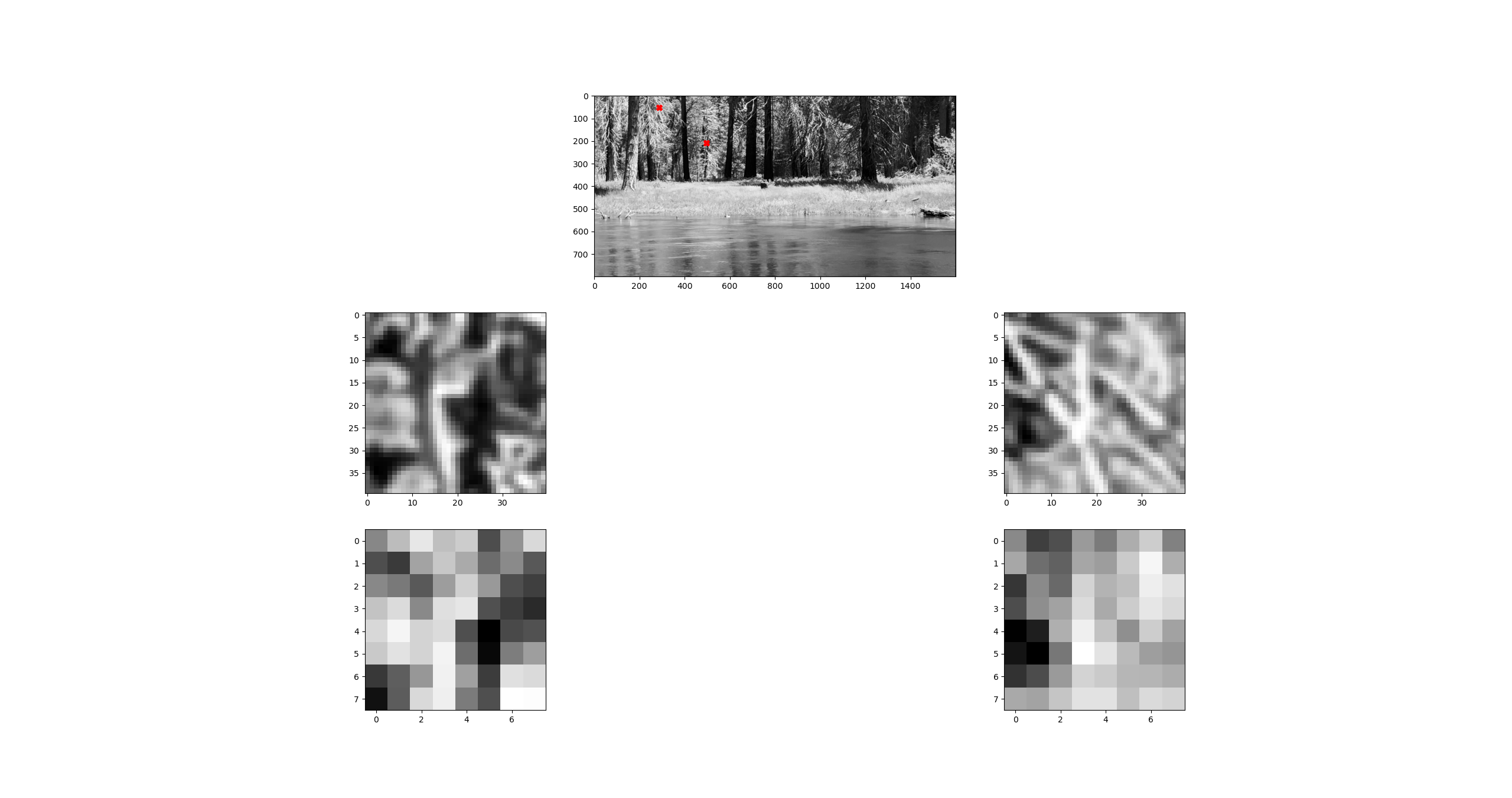
After selecting a subset of points, we treat patches around each point as a descriptor for it. We take (40, 40) patches, then blur and downsample to (8, 8). We perform bias / gain normalization so that we are considering descriptions that are invariant to affine lighting transformations.
Then we view each patch as a vector, and compute pairwise inner products between each patch. This gives a "distance" between points, that we now use for defining correspondences. For each point, we look at the ratio of (the distance to its nearest neighbor in descriptor space) and (the distance to its second nearest neighbor). If this ratio is low, it means that the pair of points in consideration are significantly more similar than the next closest in similiarity, which means that we have found a likely accurate correspondence between the points.
Now we have a decent handle on what points correspond to each other, however there will still be points that are misidentified as corresponding. To account for this, we adopt the approach for computing homgraphies. Now, the presence of bad outliers in the set of correspondences means that a least squares estimate will be pulled away from the correct homography. But we would ieally like to find the "correct" homography. To do so, we employ the RANSAC method. This is a powerful method that exemplifies the "robustness through noise" paradigm. The idea is to successively select 4 subsets of corrsponding points, compute the homography that maps from one side of the correspondence to the other, and then evaluate how well this homography explains the transformations undergone by the rest of the points. Specifically, we apply the proposed homography to all source points, and compute how many get mapped epsilon close to their corresponding point. This turns out to be an extremely effective approach, while also being beautifully simple!
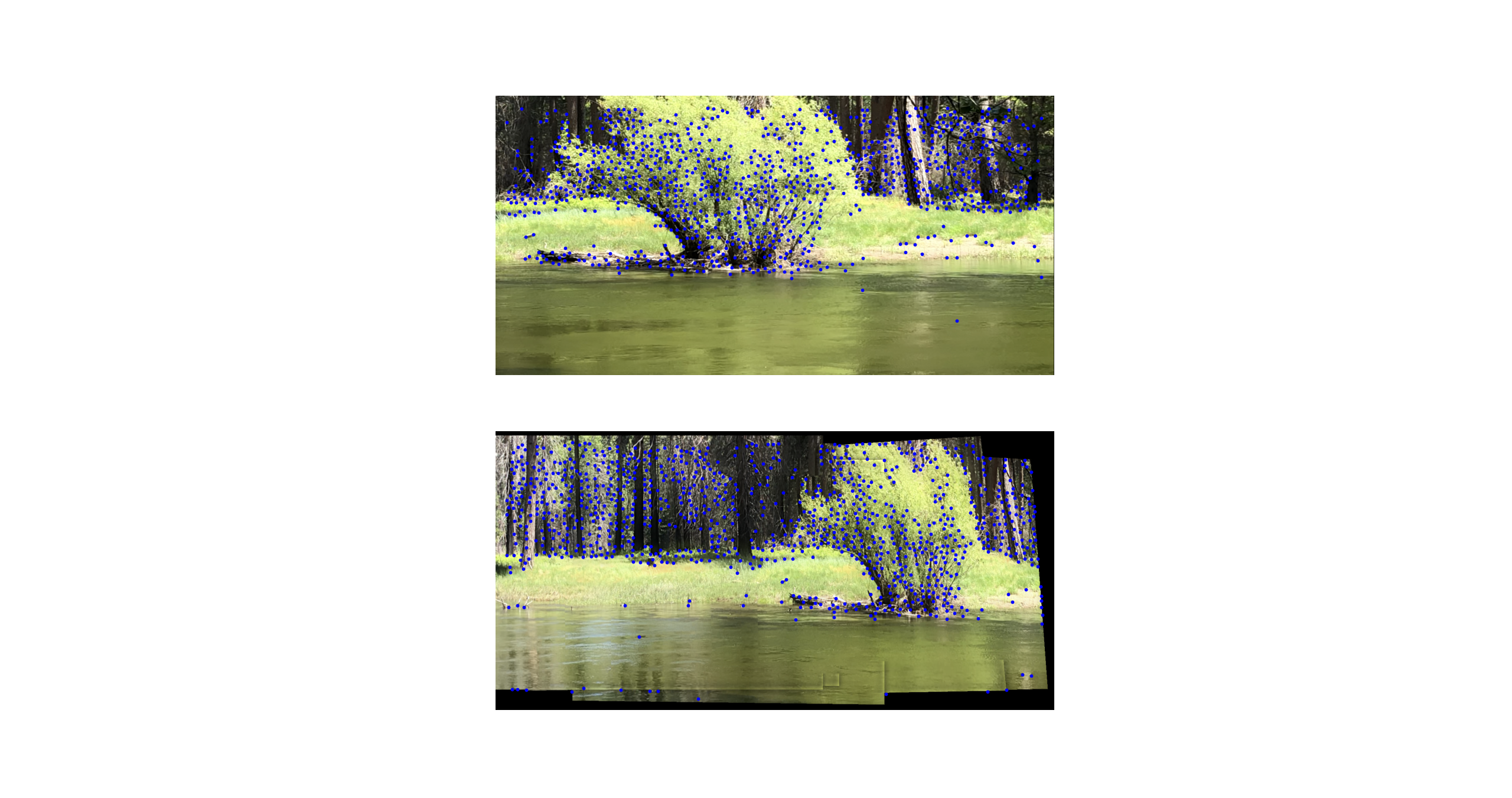
Now we have automatic correspondences implemented, we can stitch together some larger panoramas.